(See Practical
Matters at the end of this chapter.)(state) to the inputs that
must be generated to obtain the necessary behavior. +
is the next state, the equations for the four flip-flop types are+
= + = D+ =
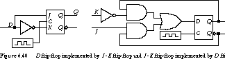
+ = As an example, Figure 6.40 shows how to implement a D flip-flop with a J-K flip-flop and, correspondingly, a
J-K flip-flop with a D flip-flop.
Consider the leftmost circuit. If D is 1, we
place the J-K flip-flop in its set input con\xde
guration (J = 1, K =
0). If D is 0, J-K's inputs are
configured for reset (J = 0, K
= 1). In the case of the rightmost circuit,
the D flip-flop's input is driven with logic that implements
the characteristic equation for the J-K flip-flop,
namely ![]() .
.
General Procedure We can follow a general procedure to map among the different kinds of flip-flops. It is based on the concept of an excitation table, that is, a table that lists all possible state transitions and the values of the flip-flop inputs that cause a given transition to take place.
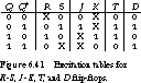
Figure 6.41 gives excitation tables for R-S,
J-K, T, and D flip-flops. If the
current state is 0 and the next state is to be 0 too, then the first
row of the table describes the flip-flop input to cause that state
transition to take place. If an R-S latch is being used,
it doesn't matter what value is placed on R as long as S
is left unasserted. R = 0, S =
0 holds the current state at 0; R = 1, S
= 0 resets the state to 0. The effect is the same.
If we are using a J-K flip-flop, the transition from 0 to 0 is accomplished by ensuring that J
is left unasserted. The value of K does not matter. If J
= 0, K = 0, the current state is held
at 0; if J = 0, K = 1, the state
is reset to 0.
If we are using a T flip-flop, the transition
does not change the current state, so the input should be 0. If a D
flip-flop is used, we set the input to the desired next state, which
is 0 in this case. The same kind of analysis can be applied to complete
the excitation table for the three other cases.
A flip-flop's next state function can be written
as a K-map. For example, the next state K-map for the
D flip-flop is shown in Figure 6.42(a).
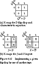
To realize a D flip-flop in terms of a J-K
flip-flop, we simply remap the state transitions implied by the D
flip-flop's K-map into equations for the J and K
inputs. In other words, we express J and K as functions
of the current state and D.
The procedure works as follows. First we draw K-maps
for J and K, as in Figure 6.42(b).
Then we fill them in the following manner. When D =
0 and Q = 0, the next state is 0. The excitation table
tells us that the inputs to J and K should be 0 and X,
respectively, if we desire a 0-to-0 transition. These values are placed
into corresponding entries of the J and K K-maps. The
inputs D = 0, Q = 1 lead to
a next state of 0. This is a 1-to-0 transition, and J and K
should be X and 1, respectively. For D = 1, Q
= 0, the transition is from 0 to 1, and J must be
1 and K should be X. The final transition, D
= 1, Q = 1, is from 1 to 1, and J
and K are X and 0. A quick look at the K-maps confirms that J = D and K =
![]() .
.
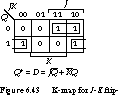
The implementation of a J-K flip-
flop by a D flip-flop follows the same procedure. We start
with a K-map to describe the next state in terms of the three variables
J, K, and the current state Q. To obtain the
transition from 0 to 0 or 1 to 0 requires that D be 0; similarly,
D must be 1 to implement a 0-to-1 or 1-to-1 transition. In other
words, the function for D is identical to the next state. The equation
for D can be read directly from the next state K-map for the J-K
flip-flop:
This K-map is shown in Figure 6.43.D =